This Rmarkdown vignette is a reimplementation of an iPython notebook created by Julia Wagemann (available here). It demonstrates how notebooks can be used for automatic geospatial report generation that ties together many different processing libraries (in this case gdal, R, and QGIS for executing processing algorithms as well as rendering).

Download & re-project shapefiles

# Madagascar
country <- "MDG"

countrywaterzip <- paste(country, "_wat.zip", sep = "")

download.file(paste("http://biogeo.ucdavis.edu/data/diva/wat/", countrywaterzip, sep = ""),
  dest = countrywaterzip)
unzip(countrywaterzip)

Load vector data into memory.

# load rgdal for readOGR()
library(rgdal)

waterlines <- readOGR(paste(country, "_water_lines_dcw.shp", sep = ""))

## OGR data source with driver: ESRI Shapefile 
## Source: "MDG_water_lines_dcw.shp", layer: "MDG_water_lines_dcw"
## with 3019 features
## It has 5 fields

waterareas <- readOGR(paste(country, "_water_areas_dcw.shp", sep = ""))

## OGR data source with driver: ESRI Shapefile 
## Source: "MDG_water_areas_dcw.shp", layer: "MDG_water_areas_dcw"
## with 338 features
## It has 5 fields

Then reproject to UTM zone 38S (EPSG:32738) to get meters as a distance unit (instead of degrees).

# load sp for CRS()
library(sp)

targetprojection <- CRS("+proj=utm +zone=38 +south +ellps=WGS84 +datum=WGS84 +units=m +no_defs")

waterlines <- spTransform(waterlines, targetprojection)
waterareas <- spTransform(waterareas, targetprojection)

Rasterise shape files

First we create a raster object with the same extent and projection as the shapefile.

library(raster)

## Loading required package: sp

r <- raster(waterlines, ncol = 4000, nrow = 8000)

Then we rasterise the water (vector) data:

# fill '1' in water areas, untouched parts stay NA
r <- rasterize(waterareas, r, field = 1)
# fill '1' along rivers, only overwrite cells which are not yet marked as water
r <- rasterize(waterlines, r, field = 1, update = TRUE, updateValue = NA)

Calculate distance to closest water source

Here we first make use of the qgisremote plugin to access the proximity processing algorithm provided by gdalogr to calculate each raster cell’s distance (in Mercator meters) to the closest water source.

library(qgisremote)

# first, add raster data to QGIS
waterlayer <- iface.addRasterLayer(r)

# create target filename for the proximity algorithm's result
proximityfile <- paste(getwd(), "waterproximity.tif", sep = "/")

# now run gdal's proximity algorithm on the data to calculate the geographic
# distance to the nearest '1' value
processing.runalg("gdalogr:proximity", INPUT = waterlayer,
  OUTPUT = proximityfile, VALUES = 1) # RTYPE = 4

Clip raster

The proximity algorithm could not distinguish between land and ocean cells, so we still need to clip the proximity raster along the country (in this case island) boundaries.

# get full country outline from GADM
outline <- raster::getData("GADM", country = country, level = 0)

It is good policy to immediately convert the polygon to the same projection to speed up the analysis/clipping.

# use [1] to select only the multipolygon without its attribute data
outline <- spTransform(outline[1], targetprojection)

rgdal::writeOGR(outline, ".", "outline", "ESRI Shapefile", overwrite_layer = TRUE)

proximity <- gdalUtils::gdalwarp(proximityfile, "waterproximityclipped.tif",
  cutline = "outline.shp", overwrite = TRUE, output_Raster = TRUE)

Equivalently, we could be doing the same thing in (R) memory using the mask() function from the raster package (although it does appear to take quite a bit longer than using gdalwarp()).

# inverse = TRUE sets those values to NA which are NOT covered by the outline polygon
proximity <- raster::mask(raster::raster(proximityfile), outline, inverse = TRUE)

Plot resulting raster

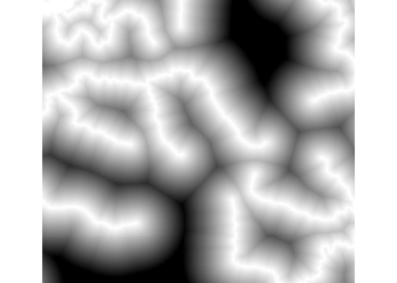
While we could simply do plotting in R based on the resulting proximity RasterBrick, let’s use the QGIS map canvas methods instead:

iface.newProject()
layer <- iface.addRasterLayer(proximity)

mapCanvas.zoomToFullExtent()
raster::plotRGB(mapCanvas.saveAsImage())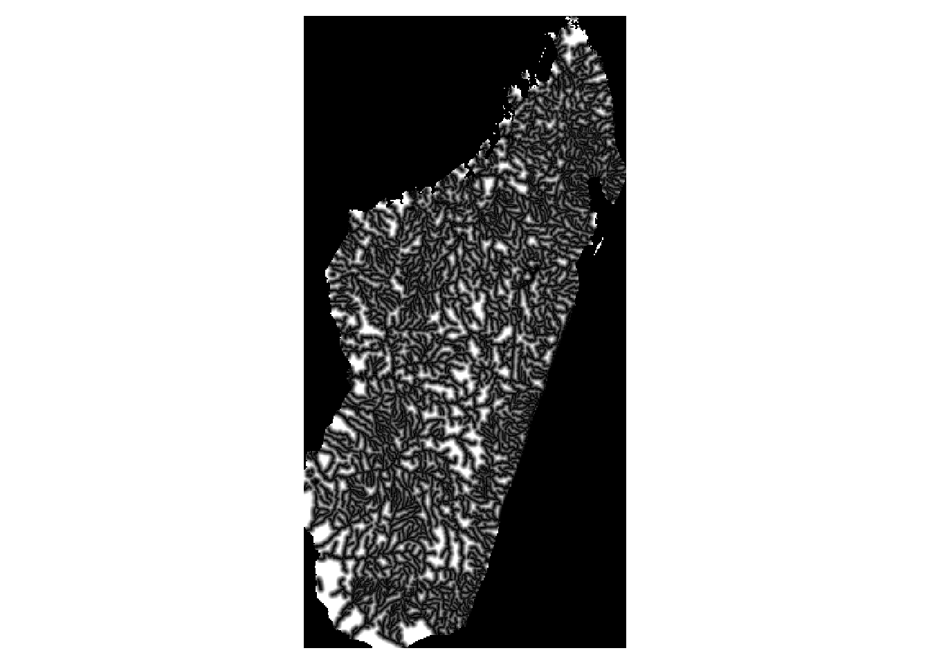

Set map canvas projection to lat/lon so we can zoom in using geographical coordinates:

mapCanvas.setCrsTransformEnabled(TRUE)

## [1] TRUE

mapCanvas.setDestinationCrs('EPSG:4326')

## CRS arguments:
##  +proj=longlat +datum=WGS84 +no_defs +ellps=WGS84 +towgs84=0,0,0

mapCanvas.setExtent(c(46.85, -19.65, 47.33, -19.07))

## [1] 3.956906

raster::plotRGB(mapCanvas.saveAsImage())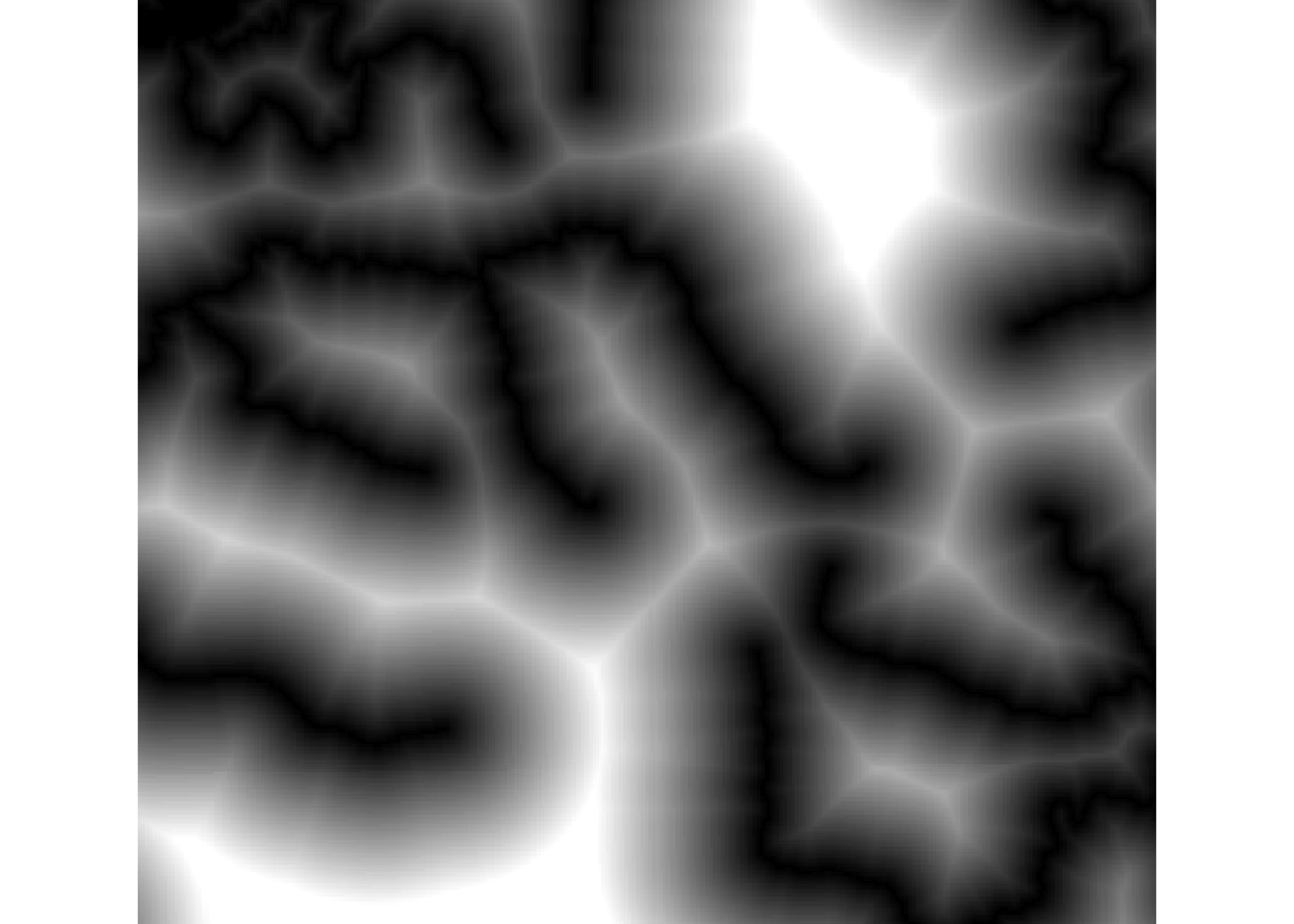

The default (single band grayscale) rendition can now be edited using the qgisxml() function (see the rendering tutorial):

r <- mapLayer.renderer(layer)
qgisxml(r)

##             name  attrname          value
## 1 rasterrenderer  gradient   BlackToWhite
## 2 rasterrenderer   opacity              1
## 3 rasterrenderer alphaBand             -1
## 4 rasterrenderer      type singlebandgray
## 5 rasterrenderer  grayBand              1

qgisxml(r, 'gradient') <- 'WhiteToBlack'
mapLayer.renderer(layer) <- r

raster::plotRGB(mapCanvas.saveAsImage())